
В статистике регрессия — это метод, который можно использовать для анализа взаимосвязи между переменными-предикторами и переменной-откликом.
Когда вы используете программное обеспечение (например, R, SAS, SPSS и т. д.) для выполнения регрессионного анализа, вы получите в качестве выходных данных таблицу регрессии, в которой суммируются результаты регрессии. Важно уметь читать эту таблицу, чтобы понимать результаты регрессионного анализа.
В этом руководстве рассматривается пример регрессионного анализа и дается подробное объяснение того, как читать и интерпретировать выходные данные таблицы регрессии.
Пример регрессии
Предположим, у нас есть следующий набор данных, который показывает общее количество часов обучения, общее количество сданных подготовительных экзаменов и итоговый балл за экзамен, полученный для 12 разных студентов:

Чтобы проанализировать взаимосвязь между учебными часами и сданными подготовительными экзаменами и окончательным экзаменационным баллом, который получает студент, мы запускаем множественную линейную регрессию, используя отработанные часы и подготовительные экзамены, взятые в качестве переменных-предикторов, и итоговый экзаменационный балл в качестве переменной ответа.
Мы получаем следующий вывод:

Проверка соответствия модели
В первом разделе показано несколько различных чисел, которые измеряют соответствие регрессионной модели, т. е. насколько хорошо регрессионная модель способна «соответствовать» набору данных.

Вот как интерпретировать каждое из чисел в этом разделе:
Несколько R
Это коэффициент корреляции.Он измеряет силу линейной зависимости между переменными-предикторами и переменной отклика. R, кратный 1, указывает на идеальную линейную зависимость, тогда как R, кратный 0, указывает на отсутствие какой-либо линейной зависимости. Кратный R — это квадратный корень из R-квадрата (см. ниже).
В этом примере множитель R равен 0,72855 , что указывает на довольно сильную линейную зависимость между предикторами часов обучения и подготовительных экзаменов и итоговой оценкой экзаменационной переменной ответа.
R-квадрат
Его часто записывают как r 2 , а также называют коэффициентом детерминации.Это доля дисперсии переменной отклика, которая может быть объяснена предикторной переменной.
Значение для R-квадрата может варьироваться от 0 до 1. Значение 0 указывает, что переменная отклика вообще не может быть объяснена предикторной переменной. Значение 1 указывает, что переменная отклика может быть полностью объяснена без ошибок с помощью переменной-предиктора.
В этом примере R-квадрат равен 0,5307 , что указывает на то, что 53,07% дисперсии итоговых экзаменационных баллов можно объяснить количеством часов обучения и количеством сданных подготовительных экзаменов.
Связанный: Что такое хорошее значение R-квадрата?
Скорректированный R-квадрат
Это модифицированная версия R-квадрата, которая была скорректирована с учетом количества предикторов в модели. Он всегда ниже R-квадрата. Скорректированный R-квадрат может быть полезен для сравнения соответствия различных моделей регрессии друг другу.
В этом примере скорректированный R-квадрат равен 0,4265.
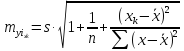
Стандартная ошибка регрессии
Стандартная ошибка регрессии — это среднее расстояние, на которое наблюдаемые значения отклоняются от линии регрессии. В этом примере наблюдаемые значения отклоняются от линии регрессии в среднем на 7,3267 единиц.
Связанный: Понимание стандартной ошибки регрессии
Наблюдения
Это просто количество наблюдений в нашем наборе данных. В этом примере общее количество наблюдений равно 12 .
Тестирование общей значимости регрессионной модели
В следующем разделе показаны степени свободы, сумма квадратов, средние квадраты, F-статистика и общая значимость регрессионной модели.

Вот как интерпретировать каждое из чисел в этом разделе:
Степени свободы регрессии
Это число равно: количеству коэффициентов регрессии — 1. В этом примере у нас есть член пересечения и две переменные-предикторы, поэтому у нас всего три коэффициента регрессии, что означает, что степени свободы регрессии равны 3 — 1 = 2 .
Всего степеней свободы
Это число равно: количество наблюдений – 1. В данном примере у нас 12 наблюдений, поэтому общее количество степеней свободы 12 – 1 = 11 .
Остаточные степени свободы
Это число равно: общая df – регрессионная df.В этом примере остаточные степени свободы 11 – 2 = 9 .
Средние квадраты
Средние квадраты регрессии рассчитываются как регрессия SS / регрессия df.В этом примере регрессия MS = 546,53308/2 = 273,2665 .
Остаточные средние квадраты вычисляются как остаточный SS / остаточный df.В этом примере остаточная MS = 483,1335/9 = 53,68151 .
F Статистика
Статистика f рассчитывается как регрессия MS/остаточная MS. Эта статистика показывает, обеспечивает ли регрессионная модель лучшее соответствие данным, чем модель, которая не содержит независимых переменных.
По сути, он проверяет, полезна ли регрессионная модель в целом. Как правило, если ни одна из переменных-предикторов в модели не является статистически значимой, общая F-статистика также не является статистически значимой.
В этом примере статистика F равна 273,2665/53,68151 = 5,09 .
Значение F (P-значение)
Последнее значение в таблице — это p-значение, связанное со статистикой F. Чтобы увидеть, значима ли общая модель регрессии, вы можете сравнить p-значение с уровнем значимости; распространенные варианты: 0,01, 0,05 и 0,10.
Если p-значение меньше уровня значимости, имеется достаточно доказательств, чтобы сделать вывод о том, что регрессионная модель лучше соответствует данным, чем модель без переменных-предикторов. Этот вывод хорош, потому что он означает, что переменные-предикторы в модели действительно улучшают соответствие модели.
В этом примере p-значение равно 0,033 , что меньше обычного уровня значимости 0,05. Это указывает на то, что регрессионная модель в целом статистически значима, т. е. модель лучше соответствует данным, чем модель без переменных-предикторов.
Тестирование общей значимости регрессионной модели
В последнем разделе показаны оценки коэффициентов, стандартная ошибка оценок, t-stat, p-значения и доверительные интервалы для каждого термина в регрессионной модели.

Вот как интерпретировать каждое из чисел в этом разделе:
Коэффициенты
Коэффициенты дают нам числа, необходимые для записи оценочного уравнения регрессии:
у шляпа знак равно б 0 + б 1 Икс 1 + б 2 Икс 2 .
В этом примере расчетное уравнение регрессии имеет вид:
итоговый балл за экзамен = 66,99 + 1,299 (часы обучения) + 1,117 (подготовительные экзамены)
Каждый отдельный коэффициент интерпретируется как среднее увеличение переменной отклика на каждую единицу увеличения данной переменной-предиктора при условии, что все остальные переменные-предикторы остаются постоянными. Например, для каждого дополнительного часа обучения среднее ожидаемое увеличение итогового экзаменационного балла составляет 1,299 балла при условии, что количество сданных подготовительных экзаменов остается постоянным.
Перехват интерпретируется как ожидаемый средний итоговый балл за экзамен для студента, который учится ноль часов и не сдает подготовительных экзаменов. В этом примере ожидается, что учащийся наберет 66,99 балла, если он будет заниматься ноль часов и не сдавать подготовительных экзаменов. Однако будьте осторожны при интерпретации перехвата выходных данных регрессии, потому что это не всегда имеет смысл.
Например, в некоторых случаях точка пересечения может оказаться отрицательным числом, что часто не имеет очевидной интерпретации. Это не означает, что модель неверна, это просто означает, что перехват сам по себе не должен интерпретироваться как означающий что-либо.
Стандартная ошибка, t-статистика и p-значения
Стандартная ошибка — это мера неопределенности оценки коэффициента для каждой переменной.
t-stat — это просто коэффициент, деленный на стандартную ошибку. Например, t-stat для часов обучения составляет 1,299 / 0,417 = 3,117.
В следующем столбце показано значение p, связанное с t-stat. Это число говорит нам, является ли данная переменная отклика значимой в модели. В этом примере мы видим, что значение p для часов обучения равно 0,012, а значение p для подготовительных экзаменов равно 0,304. Это указывает на то, что количество учебных часов является важным предиктором итогового экзаменационного балла, а количество подготовительных экзаменов — нет.
Доверительный интервал для оценок коэффициентов
В последних двух столбцах таблицы представлены нижняя и верхняя границы 95% доверительного интервала для оценок коэффициентов.
Например, оценка коэффициента для часов обучения составляет 1,299, но вокруг этой оценки есть некоторая неопределенность. Мы никогда не можем знать наверняка, является ли это точным коэффициентом. Таким образом, 95-процентный доверительный интервал дает нам диапазон вероятных значений истинного коэффициента.
В этом случае 95% доверительный интервал для часов обучения составляет (0,356, 2,24). Обратите внимание, что этот доверительный интервал не содержит числа «0», что означает, что мы вполне уверены, что истинное значение коэффициента часов обучения не равно нулю, т. е. является положительным числом.
Напротив, 95% доверительный интервал для Prep Exams составляет (-1,201, 3,436). Обратите внимание, что этот доверительный интервал действительно содержит число «0», что означает, что истинное значение коэффициента подготовительных экзаменов может быть равно нулю, т. е. несущественно для прогнозирования результатов итоговых экзаменов.
Дополнительные ресурсы
Понимание нулевой гипотезы для линейной регрессии
Понимание F-теста общей значимости в регрессии
Как сообщить о результатах регрессии
В
линейной регрессии обычно оценивается
значимость не только уравнения в целом,
но и отдельных его параметров. С этой
целью по каждому из параметров определяется
его стандартная ошибка: тb
и
та.
Стандартная
ошибка коэффициента регрессии параметра
b
рассчитывается
по формуле:
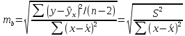
Где

остаточная дисперсия на одну степень
свободы.
Отношение
коэффициента регрессии к его стандартной
ошибке дает t-статистику,
которая подчиняется статистике Стьюдента
при

степенях
свободы. Эта статистика применяется
для проверки статистической значимости
коэффициента регрессии и для расчета
его доверительных интервалов.
Для
оценки значимости коэффициента регрессии
его величину сравнивают с его стандартной
ошибкой, т.е. определяют фактическое
значение t-критерия
Стьюдента:
 ,
,
которое затем сравнивают с табличным
значением при определенном уровне
значимостиα
и
числе степеней свободы
 .
.
Справедливо
равенство

Доверительный
интервал для коэффициента регрессии
определяется как
 .
.
Стандартная
ошибка параметра а
определяется
по формуле
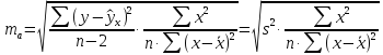
Процедура
оценивания значимости данного параметра
не отличается от рассмотренной выше
для коэффициента регрессии: вычисляется
t-критерий:

Его
величина сравнивается с табличным
значением при

степенях свободы.
Значимость
линейного коэффициента корреляции
проверяется на основе величины ошибки
коэффициента корреляции mr:

Фактическое
значение t-критерия
Стьюдента определяется как
Данная
формула свидетельствует, что в парной
линейной регрессии
 ,
,
ибо как уже указывалось,
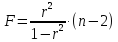 .
.
Кроме того, ,
,
следовательно, .
.
Таким
образом, проверка гипотез о значимости
коэффициентов регрессии и корреляции
равносильна проверке гипотезы о
значимости линейного уравнения регрессии.
Рассмотренную
формулу оценки коэффициента корреляции
рекомендуется применять при большом
числе наблюдений, а также если r
не близко к +1 или –1.
2.3 Интервальный прогноз на основе линейного уравнения регрессии
В
прогнозных расчетах по уравнению
регрессии определяется предсказываемое
yр
значение
как точечный прогноз
 х
х
при
хр
= хk
т.
е. путем подстановки в линейное уравнение
регрессии

соответствующего
значения х.
Однако
точечный прогноз явно нереален, поэтому
он дополняется расчетом стандартной
ошибки
 х,
х,
т.
е.
 ,
,
и
соответственно мы получаем интервальную
оценку прогнозного значения у*:
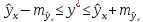
Считая,
что прогнозное значение фактора хр
= хk
получим
следующую формулу расчета стандартной
ошибки предсказываемого по линии
регрессии значения, т. е.

имеет выражение:
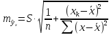
Рассмотренная
формула стандартной ошибки предсказываемого
среднего значения у
при
заданном значении хk
характеризует
ошибку положения линии регрессии.
Величина стандартной ошибки
 достигает
минимума при
и
возрастает по мере того, как «удаляется»
от
 в любом направлении. Иными словами, чем
больше разность между и
и ,
,
тем больше ошибка ,
,
с
которой предсказывается среднее значение
у
для
заданного значения
 .
.
Можно ожидать наилучшие результаты
прогноза, если признак-фактор х находится
в центре области наблюдений х, и нельзя
ожидать хороших результатов прогноза
при удалении .
.
от . Если же значение
 .
.
оказывается за пределами наблюдаемых
значенийх,
используемых при построении линейной
регрессии, то результаты прогноза
ухудшаются в зависимости от того,
насколько
 .
.
отклоняется от области наблюдаемых
значений факторах.
На
графике, приведенном на рис. 1, доверительные
границы для

представляют
собой гиперболы, расположенные по обе
стороны от линии регрессии. Рис. 1
показывает, как изменяются пределы в
зависимости от изменения
 .:
.:
две гиперболы по обе стороны от линии
регрессии определяют 95 %-ные доверительные
интервалы для среднего значенияу
при
заданном значении х.
Однако
фактические значения у
варьируют
около среднего значения
 .
.
Индивидуальные
значения у
могут
отклоняться от

на
величину случайной ошибки ε, дисперсия
которой оценивается как остаточная
дисперсия на одну степень свободы
 .
.
Поэтому ошибка предсказываемого
индивидуального значенияу
должна включать не только стандартную
ошибку
 ,
,
но и случайную ошибкуs.
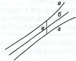
Рис.
1. Доверительный интервал линии регрессии:
а
— верхняя
доверительная граница; б
— линия
регрессии;
в
— доверительный
интервал для

при
 ;
;
г
— нижняя
доверительная граница.
Средняя
ошибка прогнозируемого индивидуального
значения у
составит:
При
прогнозировании на основе уравнения
регрессии следует помнить, что величина
прогноза зависит не только от стандартной
ошибки индивидуального значения у,
но
и от точности прогноза значения фактора
х.
Его
величина может задаваться на основе
анализа других моделей исходя из
конкретной ситуации, а также анализа
динамики данного фактора.
Рассмотренная
формула средней ошибки индивидуального
значения признака у
 может
может
быть использована также для оценки
существенности различия предсказываемого
значения и некоторого гипотетического
значения.
11
Соседние файлы в предмете [НЕСОРТИРОВАННОЕ]
- #
- #
- #
- #
- #
- #
- #
- #
- #
- #
- #
When the regression coefficients are equal to the structural coefficients, the regression residuals (the difference between the predicted and actual values of Y) can be interpreted as due to unmeasured causes of Y, and hence are equal to error terms under a causal interpretation.
From: Philosophy of Statistics, 2011
Confidence Intervals
George W. Burruss, Timothy M. Bray, in Encyclopedia of Social Measurement, 2005
Calculating Confidence Intervals for Linear Regression
Regression coefficients represent point estimates that are multiplied by values of variables to predict the dependent variable. Recall that the multiple linear regression equation is
Y=α+b1X1+b2X2+…+bkXk,
where Y is the dependent variable, X1 through Xk are values of the independent variables, α is the intercept, and b1 through bk are the regression coefficients. Unlike means and proportions, regression coefficients represent their independent effect on the dependent variable after controlling for the impact of other independent variables. First, the standard error of the regression coefficient is calculated as
s.e.bk=s.e.RsXkn−1,
where s.e.R is the standard deviation of the regression line (called the “standard error of the estimate” in some computer regression output data), sXk is the standard deviation of Xk, and n is the sample size.
Once the standard error has been calculated, calculating the confidence interval is straightforward. The regression coefficient is added and subtracted from the product of the associated value from the t distribution by the standard error of the regression coefficient:
bk±tα(s.e.b).
The value associated with the chosen confidence level is found in the table for t distributions at the α − 1 by n − 2 degrees of freedom.
As an example for regression coefficient confidence intervals, consider the following factors hypothesized to affect state homicide rates in 1990. Two variables are considered as correlates of homicide: percentage of a state population that has female-headed households (FEMALEHOUSE) and a state’s percentage population change in the decade preceding 1990 (POPGROWTH). The standard error of the regression line (s.e.R) is 2.105. The regression coefficients and standard output are shown in Table I. For FEMALEHOUSE, the standard error for the coefficient is calculated as
s.e.b1=2.1052.00450−1=0.150.
The standard error is then multiplied to the associated value from the t distribution (a 0.05 alpha level at 49 degrees of freedom, which is approximately 2). This product is then added to and subtracted from the regression coefficient to get the confidence interval:
1.616±2.000(0.150)=1.616±0.300or(1.316,1.916).
Thus, a 1% increase in a state’s number of female-headed households, controlling for the preceding decade’s population growth, will increase the state’s number of homicides by 1.616 per 100,000 persons, plus or minus 0.30 homicides per 100,000 persons. Note in the standard output that the FEMALEHOUSE coefficient is designated statistically significant: the p-value is 0.000. This can be also be deduced from the confidence interval; it does not contain zero, the null value, within the interval. Had the lower limit of the confidence interval been negative and the upper limit positive, the coefficient would not be considered statistically significant: the percentage of female-headed households within a state may have no (that is, zero) effect on the homicide rate.
Table I. Factors Affecting State Homicide Rates in 1990a
| Variable | b | s.e.b | p-Value | s.d.c | 95% confidence intervals | |
|---|---|---|---|---|---|---|
| Lower bound | Upper bound | |||||
| Constant | −11.128 | 1.677 | 0.000 | — | −14.503 | −7.754 |
| FEMALEHOUSE | 1.616 | 0.150 | 0.000 | 2.003 | 1.314 | 1.918 |
| POPGROWTH | 0.070 | 0.026 | 0.009 | 11.527 | 0.018 | 0.123 |
- a
- Homicide data are from the United States Federal Bureau of Investigation. The data for percentage population growth and percentage of female-headed households in the United States are from the United States Census Bureau.
- b
- Standard error.
- c
- Standard deviation.
Calculating the constant would be the same as for the regression coefficients, except for using a different formula for the constant’s standard error. Because the constant is seldom used in evaluating the regression model, no example is presented here. However, the constant is used in prediction with the regression model. The uncertainty that surrounds both the regression coefficients and the constant should be indicated in the presentation of any quantity of interest, such as a state’s predicted homicide rate. Such presentation of statistical analysis is covered in the next section.
Read full chapter
URL:
https://www.sciencedirect.com/science/article/pii/B0123693985000608
Multiple Regression
Andrew F. Siegel, Michael R. Wagner, in Practical Business Statistics (Eighth Edition), 2022
Interpreting the Regression Coefficients
The regression coefficients are interpreted as the effect of each variable on page costs, if all of the other explanatory variables are held constant. This is often “adjusting for” or “controlling for” the other explanatory variables. Because of this, the regression coefficient for an X variable may change (sometimes considerably) when other X variables are included or dropped from the analysis. In particular, each regression coefficient gives you the average increase in page costs per increase of 1 in its X variable, where 1 refers to one unit of whatever that X variable measures.
The regression coefficient for audience, b1 = 10.73, indicates that, all else being equal, a magazine with an extra 1000 readers (because X1 is given in thousands in the original data set) will charge an extra $10.73 (on average) for a one-page ad. You can also think of it as meaning that each extra reader is worth $0.01073, just over a penny per person. So if a different magazine had the same percent male readership and the same median income but 3548 more people in its audience, you would expect the page costs to be 10.73 × 3.548 = $38.07 higher (on average) due to the larger audience.
The regression coefficient for percent male, b2 = −1,020, indicates that, all else being equal, a magazine with an extra 1% of male readers would charge $1020 less (on average) for a full-page color ad. This suggests that women readers are more valuable than men readers. Statistical inference will confirm or deny this hypothesis by comparing the size of this effect (ie, −$1020) to what you might expect to find here due to random coincidence alone.
The regression coefficient for income, b3 = −1.32, indicates that, all else being equal, a magazine with an extra dollar of median income among its readers would charge about $1.32 less (on average) for a full-page ad. The sign (negative) is questionable because we would expect that people with more income can spend more on advertised products—we will subsequently explore if this effect is reasonably due to pure chance. For now, we interpret this coefficient: If a magazine had the same audience and percent male readership but had a median income $4000 higher, you would expect the page costs to be −1.32 × 4000 = −$5280 lower (on average) due to the higher income level.
Remember that regression coefficients indicate the effect of one X variable on Y while all other X variables are held constant. This should be taken literally. For example, the regression coefficient b1 indicates the effect of audience size on page costs, computed while holding median income and percent male readership fixed. In this example, higher audience levels tend to result in higher page costs at fixed levels of median income and of male readership (due to the fact that b1 is a positive number).
What would the relationship be if the other variables, audience and percent male, were not held constant? This may be answered by looking at the ordinary correlation coefficient (or regression coefficient predicting Y from this X alone), computed for just the two variables: page costs and median income. In this case, higher median income is actually associated with lower page costs (the correlation of page costs with median income is negative: −0.40)! How can this be? One reasonable explanation is that magazines targeting a higher median income level cannot support a large audience due to a relative scarcity of rich people in the general population, and this is supported by the negative correlation (−0.30) of audience size with median income. If this audience decrease is large enough, it can offset the effect of higher income per reader, which can support the negative b3 coefficient for median income observed earlier.
Read full chapter
URL:
https://www.sciencedirect.com/science/article/pii/B9780128200254000129
Linear Regression
Ronald N. Forthofer, … Mike Hernandez, in Biostatistics (Second Edition), 2007
13.4.1 The Multiple Linear Regression Model
The equation showing the hypothesized relation between the dependent and (p − 1) independent variables is
yi=β0+β1x1i+β2 x2i+⋯+βp-1xp-1,i+ɛi.
The coefficient βi describes how much change there is in the dependent variable when the ith independent variable changes by one unit and the other independent variables are held constant. Again, the key hypothesis is whether or not βi is equal to zero. If βi is equal to zero, we probably would drop the corresponding Xi from the equation because there is no linear relation between Xi and the dependent variable once the other independent variables are taken into account.
The regression coefficients of (p − 1) independent variables and the intercept can be estimated by the least squares method, the same approach we used in the simple model presented above. We are also making the same assumptions — independence, normality, and constant variance — about the dependent variable and the error term in this model as we did in the simple linear regression model. We can also partition the sums of squares for the multiple regression model similarly to the partition used in the simple linear regression situation. The corresponding ANOVA table is
| Source | DF | Sum of Squares | Mean Square | F-ratio |
|---|---|---|---|---|
| Regression | p − 1 | ∑ (ŷi − 2 ) = SSR | SSR/(p − 1) = MSR | MSR/MSE |
| Residual | n − p | ∑ (yi − ŷi )2 = SSE | SSE/(n p) MSE | |
| Total | n − 1 | ∑ ( yi − 2) |
and the overall F ratio now tests the hypothesis that the p − 1 regression coefficients (excluding the intercept) are equal to zero.
A goal of multiple regression is to obtain a small set of independent variables that makes sense substantively and that does a reasonable job in accounting for the variation in the dependent variable. Often we have a large number of variables as candidates for the independent variables, and our job is to reduce that larger set to a parsimonious set of variables. As we just saw, we do not want to retain a variable in the equation if it is not making a contribution. Inclusion of redundant or noncontributing variables increases the standard errors of the other variables and may also make it more difficult to discern the true relationship among the variables. A number of approaches have been developed to aid in the selection of the independent variables, and we show a few of these approaches.
The calculations and the details of multiple linear regression are much more than we can cover in this text. For more information on this topic, see books by Kleinbaum, Kupper, and Muller and by Draper and Smith, both excellent texts that focus on linear regression methods. We consider examples for the use of multiple linear regression based on NHANES III sample data that are shown in Table 13.6.
Table 13.6. Adult (=18 years of age) sample data from NHANES III, Phase II (1991–1994).
| Row | Racea | Sexb | Agec | Educationd | Heighte | Weightf | Smokeg | SBPh | BMIi |
|---|---|---|---|---|---|---|---|---|---|
| 1 | 1 | 1 | 28 | 16 | 68 | 160 | 7 | 111 | 24.33 |
| 2 | 1 | 1 | 26 | 12 | 68 | 165 | 1 | 101 | 25.09 |
| 3 | 2 | 2 | 31 | 15 | 68 | 175 | 1 | 120 | 26.61 |
| 4 | 2 | 1 | 18 | 12 | 76 | 265 | 7 | 158 | 32.26 |
| 5 | 1 | 1 | 50 | 17 | 67 | 145 | 1 | 125 | 22.71 |
| 6 | 2 | 1 | 42 | 12 | 69 | 247 | 1 | 166 | 36.48 |
| 7 | 1 | 2 | 20 | 12 | 66 | 156 | 7 | 114 | 25.18 |
| 8 | 1 | 1 | 29 | 12 | 76 | 180 | 1 | 143 | 21.91 |
| 9 | 1 | 2 | 35 | 12 | 63 | 166 | 2 | 111 | 29.41 |
| 10 | 1 | 1 | 47 | 16 | 66 | 169 | 1 | 133 | 27.28 |
| 11 | 1 | 2 | 20 | 14 | 69 | 120 | 7 | 95 | 17.72 |
| 12 | 1 | 2 | 33 | 16 | 68 | 133 | 7 | 113 | 20.22 |
| 13 | 4 | 1 | 24 | 13 | 71 | 185 | 7 | 128 | 25.80 |
| 14 | 1 | 1 | 28 | 14 | 72 | 150 | 1 | 110 | 20.34 |
| 15 | 1 | 2 | 32 | 8 | 61 | 126 | 1 | 117 | 23.81 |
| 16 | 2 | 1 | 21 | 10 | 68 | 190 | 1 | 112 | 28.89 |
| 17 | 1 | 1 | 28 | 17 | 71 | 150 | 7 | 110 | 20.92 |
| 18 | 1 | 2 | 60 | 12 | 61 | 130 | 7 | 117 | 24.56 |
| 19 | 1 | 1 | 55 | 12 | 66 | 215 | 2 | 142 | 34.70 |
| 20 | 1 | 2 | 74 | 12 | 65 | 130 | 7 | 105 | 21.63 |
| 21 | 1 | 2 | 38 | 16 | 68 | 126 | 7 | 94 | 19.16 |
| 22 | 1 | 1 | 26 | 14 | 66 | 160 | 2 | 131 | 25.82 |
| 23 | 1 | 1 | 52 | 9 | 74 | 328 | 2 | 128 | 42.11 |
| 24 | 1 | 2 | 25 | 16 | 69 | 125 | 7 | 93 | 18.46 |
| 25 | 1 | 2 | 24 | 12 | 67 | 133 | 1 | 103 | 20.83 |
| 26 | 1 | 2 | 26 | 16 | 59 | 105 | 1 | 114 | 21.21 |
| 27 | 1 | 2 | 51 | 13 | 64 | 119 | 7 | 130 | 20.43 |
| 28 | 2 | 2 | 29 | 16 | 62 | 98 | 7 | 105 | 17.92 |
| 29 | 4 | 1 | 26 | 0 | 64 | 150 | 7 | 117 | 25.75 |
| 30 | 1 | 2 | 60 | 12 | 64 | 175 | 1 | 124 | 30.04 |
| 31 | 1 | 1 | 22 | 9 | 70 | 190 | 1 | 122 | 27.26 |
| 32 | 1 | 2 | 19 | 12 | 65 | 125 | 7 | 112 | 20.80 |
| 33 | 3 | 1 | 39 | 12 | 73 | 210 | 1 | 135 | 27.71 |
| 34 | 3 | 2 | 77 | 4 | 62 | 138 | 7 | 150 | 25.24 |
| 35 | 1 | 1 | 39 | 12 | 73 | 230 | 2 | 125 | 30.34 |
| 36 | 1 | 1 | 40 | 11 | 69 | 170 | 1 | 126 | 25.10 |
| 37 | 1 | 2 | 44 | 13 | 62 | 115 | 7 | 99 | 21.03 |
| 38 | 3 | 2 | 27 | 9 | 61 | 140 | 7 | 114 | 26.45 |
| 39 | 1 | 1 | 29 | 14 | 73 | 220 | 7 | 139 | 29.03 |
| 40 | 1 | 2 | 78 | 11 | 63 | 110 | 7 | 150 | 19.49 |
| 41 | 1 | 1 | 62 | 13 | 65 | 208 | 7 | 112 | 34.61 |
| 42 | 1 | 1 | 22 | 10 | 71 | 125 | 1 | 127 | 17.43 |
| 43 | 1 | 2 | 37 | 11 | 64 | 176 | 7 | 125 | 30.21 |
| 44 | 1 | 1 | 38 | 17 | 72 | 195 | 7 | 136 | 26.45 |
| 45 | 3 | 1 | 22 | 12 | 65 | 140 | 7 | 108 | 23.30 |
| 46 | 3 | 1 | 79 | 0 | 61 | 125 | 2 | 156 | 23.62 |
| 47 | 1 | 2 | 24 | 12 | 62 | 146 | 7 | 108 | 26.70 |
| 48 | 1 | 2 | 32 | 13 | 67 | 141 | 2 | 105 | 22.08 |
| 49 | 1 | 1 | 42 | 16 | 70 | 192 | 7 | 121 | 27.55 |
| 50 | 1 | 1 | 42 | 14 | 68 | 185 | 7 | 126 | 28.13 |
- a
- (1 = white, 2 = black, 3 = Hispanic, 4 = other);
- b
- (1 = male; 2 = female);
- c
- Age in years;
- d
- Number of years of education;
- e
- Height (inches);
- f
- Weight (pounds);
- g
- (1 = current smoker, 2 = never, 7 = previous);
- h
- Systolic blood pressure (mmHg);
- i
- Body mass index
Read full chapter
URL:
https://www.sciencedirect.com/science/article/pii/B9780123694928500182
Generalized Linear Mixed Models
S. Rabe-Hesketh, A. Skrondal, in International Encyclopedia of Education (Third Edition), 2010
Conditional and Marginal Relationships
The regression coefficients in generalized linear mixed models represent conditional effects in the sense that they express comparisons holding the cluster-specific random effects (and covariates) constant. For this reason, conditional effects are sometimes referred to as cluster-specific effects. In contrast, marginal effects can be obtained by averaging the conditional expectation μij over the random effects distribution. Marginal effects express comparisons of entire sub-population strata defined by covariate values and are sometimes referred to as population-averaged effects.
In linear mixed models (identity link), the regression coefficents can be interpreted as either conditional or marginal effects. However, conditional and marginal effects differ for most other link functions. This can easily be seen for a random intercept logistic regression model with a single covariate in Figure 3. The cluster-specific, conditional relationships are shown as dotted curves with horizontal shifts due to different values of the random intercept. The population-averaged, marginal curve is obtained by averaging the conditional curves at each value of xij . We see that the marginal curve resembles a logistic curve with a smaller regression coefficient. Hence, the marginal effect of xij is smaller than the conditional effect.

Figure 3. Conditional relationships (dotted curves) and marginal relationship (solid curve) for a random intercept logistic model. From Skrondal, A. and Rabe-Hesketh, S. (2004). Generalized Latest Variable Modeling: Multilevel, Longitudinal, Structural Equation Models, Boca Raton, FL: Chapman and Hall/CRC.
The difference between conditional and marginal relationships is also visible in Figure 1, but it is much less pronounced due to the relatively small estimated random intercept variance.
Read full chapter
URL:
https://www.sciencedirect.com/science/article/pii/B9780080448947013324
Statistical Analysis of Survival Models with Bayesian Bootstrap
Jaeyong Lee, Yongdai Kim, in Recent Advances and Trends in Nonparametric Statistics, 2003
4 Proportional Hazard Model
4.1 Derivation of Bayesian Bootstrap
The argument in section 2 can be generalized to construct the BB posterior for the proportional hazard model. In addition to the model assumptions in section 2, suppose that we have covariate Zi∈ℝp,i=1,…,n, and that the distribution Fi of Xi with covariate Zi is given by 1−Fit=1−FtexpβTZi for unknown regression parameter β∈ℝp where F is the baseline distribution function. Let A be the chf of F and Ai be that of Fi, which is given by dAit=1−1−dAtexpβTZi. If A is absolutely continuous with respect to Lebesgue measure, there exists a hazard function a such that At=∫0tasds and the hazard function of Ai is ateβTZi, giving the reason why the model is called the proportional hazard model. Similar argument as in section 2 leads to the BFBB and PFBB likelihoods
LnBβA=∏t∈Tn∏i∈Dt1−(1−ΔAteβTZi)ΔNit1−ΔAt∑i∈RtDteβTZiLnPβA=∏t∈Tnexp(∑i∈DtβTZi)ΔAtΔNtexp(−ΔAt∑i∈RtexpβTZi).
Interestingly, these two forms of the likelihood were also used by frequentists too. See [14] for the BFBB likelihood and [13] for the PFBB likelihood.
We use the same prior for A as in section 2. For the prior of β, we recommend the subjective prior. But, under mild conditions one can use the improper constant prior. See [4] for a sufficient condition for the propriety of the PFBB posterior.
The BFBB posterior with prior (4) for ΔA(t) and π(β) for β is given by
(7)πβ,ΔA|Data∝LnBβA∏t∈TnΔAt−11−ΔAt−1πβ,
and the PFBB posterior of β and ΔA(t) with prior (5) for ΔA(t) and π(β) for β, is given by
(8)πβ,ΔA|Data∝πβ∏t∈Tnexp(∑i∈DtβTZi)ΔAtΔNt−1exp(−ΔAt∑i∈RteβTZi).
There is an interesting distributional structure to the PFBB posterior (8). The jump sizes ΔA(t) for t∈Tn, given β, are independent and follow
ΔAt|β,Data∼GammaΔNt,∑i∈RteβTZi.
Integrating out ΔA(t) from the PFBB posterior, we get the marginal posterior of β,
πβ|Data∝πβ∏t∈Tnexp∑i∈DtβTZi(∑i∈RtexpβTZi)ΔNt=πβ×Cox’spartiallikelihood.
When the regression coefficient β is the only parameter of interest, the PFBB gives a justification for the Bayesian analysis with the partial likelihood and a prior on β, as was done in [15].
Remark
Note that when β = 0, both BB posteriors of the proportional hazard model reduce to those of the right censored data.
Remark
Kim and Lee [4] showed that under mild conditions, both BB posterior distributions are asymptotically equivalent to the sampling distribution of the nonparametric maximum likelihood estimator.
4.2 Inference with MCMC
Inference with both BB posteriors can be done by sampling posterior samples using MCMC. In the following, we present an MCMC sampling scheme.
- •
-
Sampling β given A: In both BB posteriors, the conditional posterior distributions of β given A are not well known distributions. But, our experience shows the random walk Metropolis-Hastings sampler works reasonably well. Since the Cox’s partial likelihood is well approximated by a normal distribution, we expect that acceptance-rejection method with a normal proposal with variance an integer (typically 2 or 3) multiple of the frequentist variance estimator.
- •
-
Sampling A given β: For the PFBB, the conditional distribution of ΔA(t) given β is Gamma ΔNt,∑i∈RteβTZi. For the BFBB, random walk Metropolis-Hastings sampler works well. An alternative sampling method can be derived by modifying the algorithm of Laud, Damien and Smith [16] for the fixed jumps of the beta process posterior.
Remark
Kim and Lee [4] performed a simulation, which shows that the small sample frequentist’s property of the BFBB is better than the standard frequentist’s methods when the survival times are grouped.
Read full chapter
URL:
https://www.sciencedirect.com/science/article/pii/B9780444513786500272
Mixed-effects multinomial logit model for nominal outcomes
Xian Liu, in Methods and Applications of Longitudinal Data Analysis, 2016
11.7 Summary
As the regression coefficients of covariates in the multinomial logit model are not interpretable substantively, a supplementary procedure is to use the fixed-effect estimates to predict the probabilities marginalized at certain covariate values. This application, however, can entail serious prediction bias due to misspecification of the predictive distribution of the random components. For the mixed-effects multinomial logit model, the random components cannot be overlooked in nonlinear predictions of the marginal probabilities. If a given random component in the model is truly normally distributed, the multivariate normality on the logit scale must be retransformed to a multivariate lognormal distribution to correctly predict the response probabilities. With such retransformation, the expectation of the lognormal distribution for the multiplicative random variable is not unity but some quantity greater than one unless both the between-subjects and the within-subject random components are zero for all individuals. Additionally, without retransforming the distribution of the random components, the variance of the predicted probabilities will be much underestimated, thereby affecting the quality of significance tests on nonlinear predictions. The BLUP approach, widely applied in longitudinal data analysis, accounts for a portion of between-subjects variability in nonlinear predictions of the response probabilities. This predicting method, however, overlooks not only the dispersion of the random effect prediction but also the within-subject random errors that may exist inherently even with the specification of the between-subjects random effects. The retransformation method accounts for both between-subjects and within-subjects variability simultaneously in the construct of the mixed-effects multinomial logit model.
I would like to emphasize that from the standpoint of Bayesian inference, the posterior predictive distribution of the random components in the mixed-effects multinomial logit model is not normality but lognormality. Correspondingly, the expectation of this predictive distribution for the random effects is greater than one. In the previous illustration, I compare three sets of the predicted probabilities for three health states at six time points, obtained from three predicting approaches – the retransformation method, the empirical BLUP, and the fixed-effects model – as relative to the predictions from a specified full model. In particular, I examine how each of these methods behaves in nonlinear predictions after an important predictor variable is removed from the estimating process. The results of the empirical illustration display that failure to retransform the random effects adequately in the mixed-effects multinomial logit model results in biased longitudinal trajectories of health probabilities and considerable underestimation of the corresponding standard errors, even though the estimated regression coefficients of covariates tend to be unbiased. These biases in nonlinear predictions, in turn, can exert substantial influences on the significance tests for the effects of covariates on the predicted probabilities.
It is also shown in the illustration that after the statistically significant fixed effects of marital status on the logit scale are converted into the conditional effects on the probabilities, each of the effect estimates has a much widened dispersion on the probability scale. Consequently, at older ages, those currently married and currently not married do not display statistically significant, substantively notable differences in health probabilities at any of the time points, except for one. This loss of statistical significance is because the fixed effects are population-averaged, and therefore, the subject-specific variability is disregarded; once the random effects are introduced in prediction of the health probabilities, the inherent variability in the predictions is much increased, thereby lowering the value of the chi-square statistic. Consequently, the difference between two predicted probabilities of a given health state becomes much less likely to be statistically meaningful.
Read full chapter
URL:
https://www.sciencedirect.com/science/article/pii/B9780128013427000113
Mixed-effects regression model for binary longitudinal data
Xian Liu, in Methods and Applications of Longitudinal Data Analysis, 2016
10.9 Summary
As the regression coefficients of covariates in the mixed-effects logit model are not highly interpretable, the fixed-effect estimators are sometimes applied for nonlinear predictions. Such an application, however, can result in tremendous retransformation bias due to the neglect of retransformation of the random components. If the random components in a mixed-effects logit model are truly normally distributed, such normality needs to be retransformed to a lognormal distribution as a prior to correctly predict the response probability. Consequently, the expectation of the posterior predictive distribution for the random components is not unity in nonlinear predictions unless both the between-subjects and the within-subject random components are zero for all subjects. Furthermore, without appropriately retransforming the random components, the variance of nonlinear predictions is considerably underestimated, thereby ushering in misleading test conclusions. The best linear unbiased prediction, widely applied in longitudinal data analysis, accounts for a portion of between-subjects variability in nonlinear predictions; nevertheless, this approach overlooks within-subject variability that is present in certain situations, even in the presence of the specified random effects. The empirical illustration in this chapter displays that any neglect of retransforming of the random components can result in tremendous prediction bias. The fixed-effects perspective completely overlooks retransformation of the random components, thereby resulting in severely biased nonlinear predictions, both point and variance. By contrast, the retransformation method provides a powerful means to derive unbiased nonlinear predictions on the response probability, in which both between-subjects and within-subject variability can be appropriately modeled.
The bias in nonlinear predictions can impact significantly on the significance test for the effect of a covariate on the response probability. The above illustration displays conversion from the fixed effect of marital status on the logit scale, statistically significant, to the conditional effect on the probability of disability. The computed conditional effect is associated with a much widened dispersion on the probability scale, statistically significant only at two time points. This loss of statistical significance is thought to be because the fixed effect is population-averaged, and therefore, the subject-specific variability is disregarded; once the random effect is accounted for in computing the predicted probability, the inherent variability in nonlinear predictions is much increased, thereby lowering the value of the chi-square statistic. The retransformation method, accounting for both the between-subjects and within-subjects random components simultaneously in nonlinear predictions, is shown to yield unbiased conditional effects of covariates on the response probability. The conditional OR, displaying the effect of the covariate on a relative risk score, ignores variability in the difference between two absolute probabilities, thereby resulting in misleading prediction results on the response. Indeed, in the analysis of binary longitudinal data, considerable caution must be exercised to use the OR estimate to evaluate the results of the mixed-effects logit model.
In the application of the mixed-effects logit model, another issue worth further attention is the potential presence of selection bias in binary longitudinal data. For example, in aging and health research, it is generally perceived that frailer individuals tend to be selected out systematically in survival processes. Without accounting for this selection mechanism, the results from the mixed-effects logit model in survivors can be associated with serious selection bias. Given the impact of the inherent unobserved heterogeneity in the selection of the fittest process, the pattern of change over time in the probability of disability, as shown in the previous illustration, may be just an artifact. This issue was discussed in Chapter 7 when special topics of linear mixed models were described. In the analysis of binary longitudinal data, some statisticians recommend the use of mortality as a competing risk (Fitzmaurice et al., 2004; McCulloch et al., 2008). By specifying an additional level in the response variable, the binary longitudinal data structure becomes multinomial, and correspondingly, the mixed-effects multinomial logit model needs to be applied to find statistically efficient, consistent, and robust parameter estimates within an integrated regression process. Given the importance of analyzing longitudinal data with more than two discrete levels, Chapter 8 is devoted entirely to the mixed-effects multinomial logit model.
Read full chapter
URL:
https://www.sciencedirect.com/science/article/pii/B9780128013427000101
Volume 4
L. Coulier, … R.H. Jellema, in Comprehensive Chemometrics, 2009
4.09.5.2.1 Results
The metabolites with the 10 highest absolute regression coefficients per time point (see also Table 2) were selected from the LC-MS polar and GC-MS global n-PLS-DA models as being most discriminative between subjects treated with diclofenac and placebo. This resulted in a total of 15 metabolites from the GC-MS global data set and a total of 24 metabolites from the LC-MS polar data set for metabolite identification. Ultimately, 69% of the selected metabolites could be identified (14 out of 15 in the GC-MS global data set; 13 out of 24 in the LC-MS polar data set). Table 3 lists these most discriminating metabolites that could be identified.
Table 3. Overview of most discriminating metabolites, ranked according to their importance to the model, and their metabolite response in the OGTT time course
| Metabolite | Response type | |
|---|---|---|
| GC-MS global | Uric acid | A |
| 1,2-Diglyceride (C36:2) | A | |
| Proline | A | |
| Isoleucine | A | |
| 1-Aminocyclopentanecarboxylic acid | A | |
| Threonine | A | |
| 4-Hydroxyproline | A | |
| 2,3,4-Trihydroxybutanoic acid | A | |
| Aminoadipic acid | A | |
| Arabitol, ribitol, or xylitol | A | |
| Ornithine | A | |
| Mannose or galactose | A | |
| Palmitoleic acid (C16:1) | A | |
| Palmitic acid (C16:0) | A | |
| LC-MS polar | Isoleucine | A |
| Glycine | B | |
| 2-Amino-2-methyl butanoic acid | A | |
| 5-Oxoproline | B | |
| 1-Aminocyclopentanecarboxylic acid | A | |
| 4-Hydroxyproline | A | |
| Isoleucine and leucine (not resolved) | A | |
| Hippuric acid | A | |
| 5-Oxoproline (acetonitrile adduct) | B | |
| Aspartic acid | B | |
| Glutamic acid | B | |
| Citric acid | A |
A, contributed to treatment differences at each time point of the time course (Figure 7);
B, contributed to treatment differences in the second part of the time course (Figure 9).
Read full chapter
URL:
https://www.sciencedirect.com/science/article/pii/B9780444527011000144
Metric Predicted Variable with Multiple Metric Predictors
John K. Kruschke, in Doing Bayesian Data Analysis (Second Edition), 2015
18.4.5 Caution: Interaction variables
The preceding sections, regarding shrinkage of regression coefficients and variable selection, did not mention interactions. When considering whether to include interaction terms, there are the usual considerations with respect to inclusion of any predictor, and additional considerations specific to interaction variables.
When considering the inclusion of interaction terms, and the goal of the analysis is explanation, then the main criterion is whether it is theoretically meaningful that the effect of one predictor should depend on the level of another predictor. Inclusion of an interaction term can cause loss of precision in the estimates of the lower-order terms, especially when the interaction variable is correlated with component variables. Moreover, interpretation of interactions and their lower-order terms can be subtle, as we saw, for example, in Figure 18.9.
When interaction terms are included in a model that also has hierarchical shrinkage on regression coefficients, the interaction coefficients should not be put under the same higher-level prior distribution as the individual component coefficients, because interaction coefficients are conceptually from a different class of variables than individual components. For example, when the individual variables are truly additive, then there will be very small magnitude interaction coefficients, even with large magnitude individual regression coefficients. Thus, it could be misleading to use the method of Equation 18.5 with the hierarchical-shrinkage program of Section 18.3, because that program puts all variables’ coefficients under the same higher-level distribution. Instead, the program should be modified so that two-way interaction coefficients are under a higher-level prior that is distinct from the higher-level prior for the single-component coefficients. And, of course, different two-way interaction coefficients should be made mutually informative under a higher-level distribution only if it is meaningful to do so.
Whenever an interaction term is included in a model, it is important also to include all lower-order terms. For example, if an xi ⋅ xj interaction is included, then both of xi and xj should also be included in the model. It is also possible to include three-way interactions such as xi ⋅ xj ⋅ xk if it is theoretically meaningful to do so. A three-way interaction means that the magnitude of a two-way interaction depends on the level of a third variable. When a three-way interaction is included, it is important to include all the lower-order interactions and single predictors, including xi ⋅ xj, xi ⋅ xk, xj ⋅ xk, xi, xj, and xk. When the lower-order terms are omitted, this is artificially setting their regression coefficients to zero, and thereby distorting the posterior estimates on the other terms. For clear discussion and examples of this issue, see Braumoeller (2004) and Brambor, Clark, and Golder (2006). Thus, it would be misleading to use the method of Equation 18.5 with the variable-selection program of Section 18.4 because that program would explore models that include interactions without including the individual components. Instead, the program should be modified so that only the meaningful models are available for comparison. One way to do this is by multiplying each interaction by its own inclusion parameter and all the component inclusion parameters. For example, the interaction xjxk is multiplied by the product of inclusion parameters, δj×kδjδk. The product of these inclusion parameters can be 1 only if all three are 1. Keep in mind, however, that this also reduces the prior probability of including the interaction.
Read full chapter
URL:
https://www.sciencedirect.com/science/article/pii/B9780124058880000180
Robust Regression
Rand Wilcox, in Introduction to Robust Estimation and Hypothesis Testing (Third Edition), 2012
10.13.12 Methods Based on Ranks
Naranjo and Hettmansperger (1994) suggest estimating regression coefficients by minimizing
∑i<jcij|ri−rj|,
where the cij are (Mallows) weights given by cij = h(xi)h(xj),
h(xi)=min{1, [c/(xi−mx)′C−1(xi−mx)]a/2}.
Letting di=(xi−mx)′C−1(xi−mx), they suggest using c=med{di}+3MAD{di}, where MAD{di} means that MAD is computed using the di values, and med is the median. They report that a = 2 is effective in uncovering outliers. The quantities mx and C are the minimum volume ellipsoid estimators of location and scale described in Chapter 6. When cij ≡ 1, their method reduces to Jaeckel’s (1972) method, which minimizes a sum that is a function of the ranks of the residuals. For the one-predictor case they replace the minimum volume ellipsoid estimators mx and C with Mx = med{xi} and C = (1.483MAD{xi})2, where MAD{xi} is the median of |x1 − Mx|, … |xn − Mx|, and Mx is the median of the xi values. The resulting breakdown point appears to be at least 0.15. Evidently, this method can be used to get good control over the probability of a type I error when testing hypotheses about the regression parameters, even when the error term is heteroscedastic, but its power can be poor (Wilcox, 1995e). For rank-based diagnostic tools, see McKean, Sheather, and Hettmansperger (1990). For other results and methods based on ranks, see Cliff (1994), Dixon and McKean (1996), Hettmansperger (1984), Hettmansperger and McKean (1977), and Tableman (1990). (For results on a multivariate linear model, see Davis & McKean, 1993.)
The method derived by Hettmansperger and McKean (1977) does not protect against leverage points, but their method can be of interest when trying to detect curvature (McKean et al., 1990, 1993Mckean et al., 1990Mckean et al., 1993). Consequently, a brief discussion of their method seems warranted. Let R(yi−x′iβ) be the rank associated with the ith residual. They determine β by minimizing Jaeckel’s (1972) dispersion function given by
D(β)=∑a(R(yi−x′iβ))R(yi−x′iβ),
where
a(i)=ϕ(i/(n+1))
for a nondecreasing function ϕ defined on (0,1) such that ∫ϕ(u)du=0 and ∫ϕ2(u)du=1. Two common choices for ϕ are ϕ(u)=12(u−0.5) and ϕ(u)=sign(u−0.5). The slope parameters can be estimated by minimizing D(β), but the intercept cannot. One approach to estimating the intercept, which can be used when the error term has a skewed distribution, is to use the median of the residuals after the slope parameters have been estimated.
Another approach is to estimate β to be the vector of values that minimizes
1n∑a(R(yi−x′iβ))|ri|
(Hössjer, 1994). Hössjer shows that this estimator can be chosen with a breakdown point of 0.5, and he establishes asymptotic normality. However, Hössjer notes that poor efficiency can result with a breakdown point of 0.5 and suggests designing the method so that its breakdown point is between 0.2 and 0.3, but under normality, the asymptotic relative efficiency is only 0.56. Despite this, the method might have a practical advantage when the error term is heteroscedastic, but this has not been determined. Yet another rank-based method was derived by Chang, McKean, Naranjo, and Sheather (1999). It can have a breakdown point of 0.5, but direct comparisons with some of the better estimators in this chapter have not been made. (For some results on R estimators, see McKean & Sheather, 1991).
Read full chapter
URL:
https://www.sciencedirect.com/science/article/pii/B978012386983800010X